1. Introduction
This presentation deals with a macroscopic phenomenon that starts with a singular state where the parameters vary abruptly in the space. The phenomenon of this type appears in many fields, such as making materials, phase-field model, fluid dynamics, thermal engineering, chemical engineering, mechanical engineering and electromagnetism. It is difficult to treat this phenomenon. This phenomenon moderates with time. We can treat it within the tolerances of the parameters when the time is greater than a certain time, c. This presentation deals with solution growth of this type.
In the numerical simulation, the liquid solution is supersaturated prior to growth. A fluid flow exists in the liquid solution. A solid solution grows. This presentation shows the most main effect of fluid flow on the composition of solid phase.
This presentation shows confusing results of which we may mistake the interpretation in the simulation. The discussion was provided at an oral presentation in the conference last year [1]. The present presentation is a poster presentation and reflects the comments for the manuscript of the special issue for that previous conference. A comment for that manuscript requested that manuscript to describe the innovation of a computational method, but it has been reported in Ref. 2. This poster presentation cites the achievement of Ref. 2, answers the questions for the innovation from audience.
This research is in the field of transport phenomena. A comment for Ref. 1 stated that the content of Ref. 1 is included in a textbook. However, we need to read the textbook more carefully and understand the principle. Usually, textbooks describe the computational methods for the case when the time is sufficiently greater than c. We have not yet systematically established the computational methods for the phenomena around c. We treat this region experientially. The author inquired of The Society of Chemical Engineers, Japan a problem on solution growth around c at the previous conference [3], but the attendees could not answer the problem. After that, this problem was solved [4]. The published paper is Ref. 2. Moreover, a series of recent articles on transport phenomena [5] did not describe errors around c in chemical engineering. This region is also an unknown region in the science and engineering. We have been discovering new phenomena such as compositional variation of solid solution in crystal growth [6], micro-bubble, development of turbulence or temporary existence of electromagnetic field in electrically conductive media. This region is also related to making materials using solution growth with poorly soluble solutes in the liquid solution.
This presentation focuses on segregation of solution growth. The calculation of segregation is delicate because the boundary condition does not have fixed values on the growth interface. The basic equations on the transport phenomena of solutes in the liquid solution are the convection-diffusion equations of solutes. In many calculations of crystal growth, the mole fractions have fixed values on the growth interface, while in the calculation of segregation, not fixed values. Moreover, boundary layer thicknesses of solute mole fractions are thin in the initial stage of the growth. In conventional calculations, the results are buried under a computational error. This presentation shows this error. And we will know the right solution for the model.
2. Nomenclature
The x-axis and z-axis are defined to be parallel and perpendicular to the growth interface, respectively. The origin is defined as the center of the growth interface.
This abstract does not use superscript and subscript for symbols due to a printing reason. Then, some symbols deviate from the conventional nomenclature.
The presentation uses the conventional nomenclature, e.g., XMs*.
————
BM ( YM − YM0 ) / YM0 (-)
c the growth time such that e1( t ) < o1( t ) when t > c (s)
DL, DM the diffusion coefficients for components L and M in the liquid solution, respectively (m2/s)
e1 the relative discretization error of pL and pM (-)
e1( t ) e1 at the origin and t (-)
h the length of liquid solution in the z direction (m)
L, M the most and less affected components by fluid flow (-)
l the length of the liquid solution in the x direction (m)
o1 the tolerance of e1 (-)
o1( t ) o1 at the origin and t (-)
pL, pM ∂XL / ∂z and ∂XM / ∂z at the growth interface (m−1)
r the ratio of volume per unit atom in liquid to that in solid (-)
sqrt( ξ ) the square root of ξ ( the square root of the unit of ξ )
t a growth time (s)
u the fluid flow velocity (m/s)
XL, XM the mole fractions of components L, M in liquid phase (-)
XL( z, t ), XM( z, t ) XL and XM at x = 0, z, and t, respectively (-)
XL0, XM0 XL and XM when growth has just started (-)
XLb, XMb XL and XM just before growth, respectively (-)
YL, YM the mole fractions of components L, M in solid phase (-)
YL0, YM0 YL and YM when growth has just started, respectively (-)
∆t the time interval employed in the finite difference method (s)
∆z the mesh size in the z direction (m)
ν the kinematic viscosity of the liquid solution (m2/s)
3. Model and method
We intend to know a computational error due to the abrupt profile of mole fractions in the z direction. We have to avoid the other errors. Then, we adopt one of the simplest models. The adopted model is a one-dimensional (1-D) model with convection [7]. We deal with a ternary system. DL > DM. The liquid solution exists in the region where z > 0. h is sufficiently greater than the boundary layer thickness of XL. The temperature is uniform and constant during the growth. Liquidus line: dXM / dXL < 0.
Mass transfer through the growth interface expressed as follows:
DM ( pM ) / DL / pL
= [ r ( YM ) − XM( 0, t )] / [ r ( YL ) − XL( 0, t )]. (1)
It is calculated only at the origin.
The fluid flow transports the liquid solution retaining the initial supersaturated state to the boundary layers of solute mole fractions. We can understand the most main effect of the fluid flow on the growth. The liquid solution flows only in the x direction. An approximate convection term is added to the diffusion equations of solutes.
∂XL( z, t ) / ∂t = ( Approximate convection term for component L ) + (Diffusion term in the z direction ),
( Approximate convection term for component L ) = 2 u ( XLb - XL( z, t ) ) / l. (2)
∂XM( z, t ) / ∂t = ( Approximate convection term for component M ) + (Diffusion term in the z direction ),
( Approximate convection term for component M ) = 2 u ( XMb - XM( z, t ) ) / l. (3)
We approximate a previous experiment of InGaP growth from indium melt [6]. L = P. M = Ga. XLb = 2.8E-2. XMb = 9.5E-3. The growth temperature is 1055 K. DM / DL = 0.56. DL = 1.6E-8 m2/s. ν =1.7E-7 m2/s. h = 2.2 mm. l = 8mm. Before growth, after the liquid solution is supersaturated, the entire liquid solution is put into contact with the substrate. This motion induces a fluid flow. This flow is approximated to Stokes' first problem [8].
u = 0.2 [ erfc( 0.5 z / sqrt( ν ( 0.25 + t ) ) ) - erfc( 0.5 z / sqrt( ν t ) ) ].
Here, the units of t and u are s and m/s, respectively. The phase diagram is approximated linearly by reading that of Ref. 6. Liquidus: dXM / dXL = -6.5. Solidus: dYL / dXL = 0, dYM / dXL = -8.
We compare the result in coarse discretization with that in fine discretization. In the coarse discretization, Δz = 66 μm, Δt = 2E-2 s. This condition is employed for conventional calculation. In the fine discretization, Δz = 0.7 μm, Δt = 7E-6 s. This discretization was derived in Ref. 2. c = 0.1 s. BM denotes a normalized YM as defined in the nomenclature. The tolerance of BM = 4E-5. o1 = 4E-5.
When the growth has just started, the derivatives in Eq. 1 are infinite. Instead of Eq. 1, we use the following equation. Ref. 2 provides the detail description of the derivation.
sqrt( DM / DL ) ( XMb − XM0 ) / ( XLb − XL0 )
= [ r ( YM ) − XM0 ] / [ r ( YL ) − XL0 ].
The above equation is solved with the phase diagram implicitly.
First time step: Eqs. 2,3 are solved with finite difference method explicitly. Next, Eq.1 is solved with phase diagram implicitly.
At the time steps after the first time step, the same procedure as that at the first time step is repeated.
4. Results and discussion
4.1 The meaning of BM
This presentation deals with short growth times. We know, from mathematics, mole fractions in solid phase are approximated to be constant if fluid flow does not exist [9]. Then, BM = 0 if fluid flow does not exist. Therefore, BM shows computational errors when fluid flow does not exist, and the effect of fluid flow when the errors are sufficiently small.
4.2 Computed results
Fig. 1 is shows computed results of BM with the coarse discretization and fine discretization described in the section, 3 Model and method. Graph 1 is the result with convection in the coarse discretization. Graph 2 is the result with convection in the fine discretization. Graph 3 and 4 are, respectively, the results in the same computational conditions as Graph 1 and 2 except that fluid flow does not exist. They are employed for verifying Graph 1 and 2.
4.3 Interpretation of computed results
In the experiment, YM had lower values at t < 5 s than those at t > 5 s. The velocity of fluid flow decreases with time by the viscosity. That is, in the experiment, BM < 0 for short growth times. In Graphs 1-3, BM < 0 and it is coincident with the experiment. However, BM < 0 in Graph 3 is against the mathematics. This shows a computational error induced by the singularity of the model. It confuses the interpretation of the result. Graph 4 shows BM = 0 at t > c = 0.1 s as planned. It conforms to the mathematics.
This model corresponds to Case 1 in the presentation of the conference to be held after this school [10]. Theorems 1-4 [10] are applicable. From Theorem 4, XL increases and XM decreases on the growth interface. Then, YM decreases. That is, BM < 0.
In the model, at the growth interface, the velocity of fluid flow is zero during the growth. Then, BM starts with zero. After that, the fluid flow affects the boundary layers of mole fractions of solutes and BM decreases. The large decrease just after the growth start in Graph 1 does not show the right solution for the model. It resulted from the computational error as shown in Graph 3. Graph 2 conforms to Theorem 1 ( BM = 0 without fluid flow ) and 4. It is the right solution for the model.
5. Conclusion
The solution for the model in solution growth with fluid flow was discussed. This paper supposed an initial supersaturation of liquid solution. The model is singular at the initial growth. This singularity buried the results of conventional calculations under the error. This paper adopted a new method to satisfy the tolerance of composition in solid phase, and showed examples of a one-dimensional model to take into account a fluid flow in the liquid solution. We knew the difference between the right and not right solutions for the model, recognized this computational error when a fluid flow exists, and found we can overcome this error when a fluid flow exists.
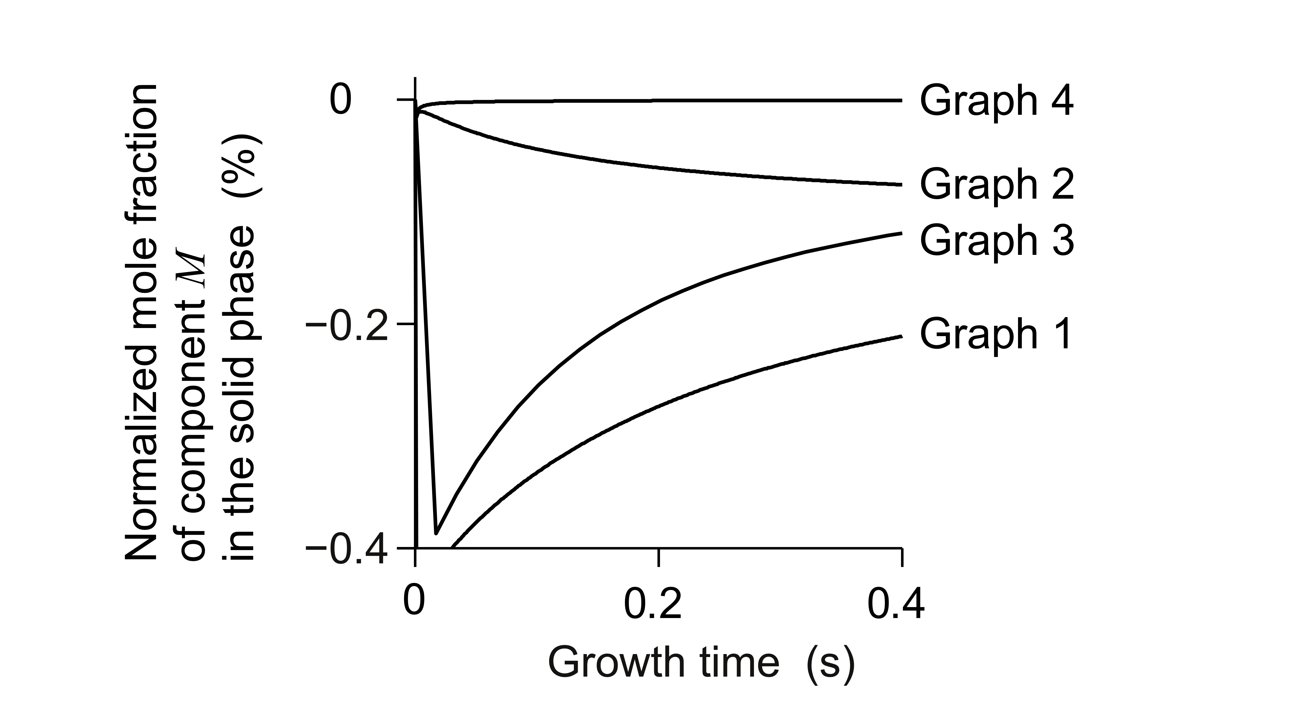
Fig. 1. The right and not right solutions for the model.
-
References
[1] H. Susawa, Proc. 7th Int. Workshop Model. Crtst. Growth, The Department of Chemical Engineering, National Taiwan University, (2011) 39-40.
[2] H. Susawa et al., Initial Condition and Calculation Method for the Numerical Simulation of LPE, J. Chem. Eng. Jpn. 40 (2007) 928-938.
[3] H. Susawa et al., Simulations of InGaP Crystal Growth by LPE Method, Soc. Chem. Eng. Jpn. 70th Annual Meeting, 70, N302 (2005) (in Japanese).
[4] H. Susawa et al., Simulation of Crystal Growth by LPE Method, Inf. Process. Soc. Jpn. Symp. Series Vol. 2005, No. 11 (2005) 323-328.
[5] S. Ookawara, Basic Lecture of Fluid Flow, Chem. Eng. Jpn., Vol. 75 No. 8-Vol. 76 No. 7 (2011-2012) (in Japanese).
[6] K. Hiramatsu et al., Jpn. J. Appl. Phys. 24 (1985) 1030–1035.
[7] H. Susawa et al., Theor. Appl. Mech. Jpn. 55 (2006) 279-284.
[8] S.Y. Leung et al., J. Cryst. Growth 60 (1982) 421–433.
[9] M. Feng et al., J. Electron. Mater. 9 (1980) 241–280.
[10] H. Susawa, Theorems for Numerical Simulation of Solution Growth with Segregation and Fluid Flow, 17th Int. Conf. Cryst. Growth Epitaxy (2013). |