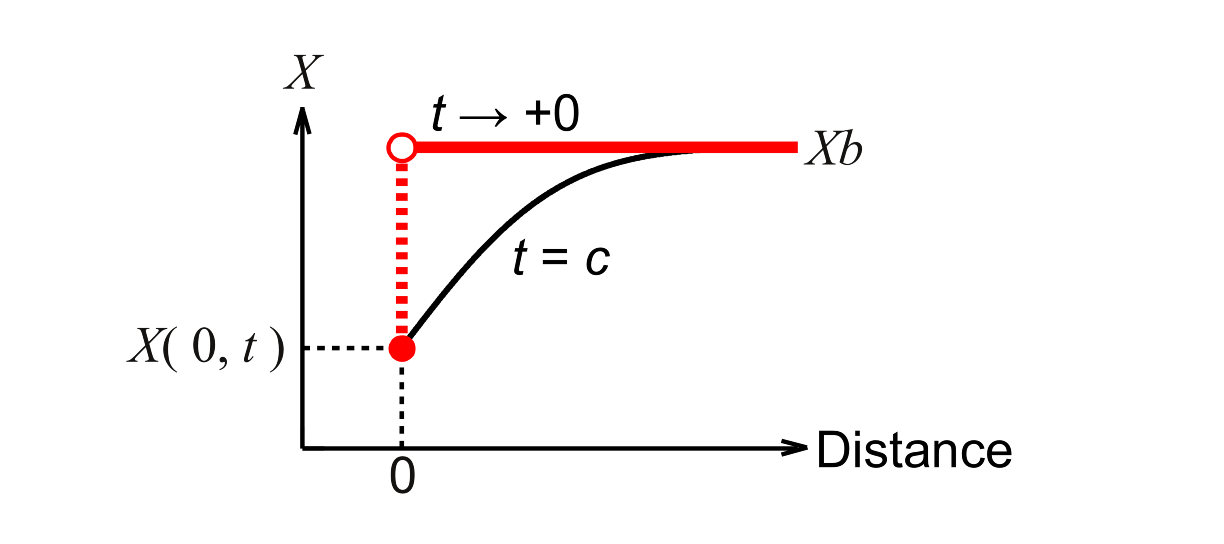
Fig. 1. A parameter varies abruptly. X denotes the parameter. t denotes a time. At t → +0, it is difficult to treat the phenomenon. At t = c, the phenomenon moderates and we can treat the phenomenon within the tolerance of parameter. In this presentation, the distance : the distance from the growth interface, t : a growth time, X : the mole fraction of a component in the liquid phase, Xb : X just before the growth, X( 0, t ) : X that is in an equilibrium state with the solid phase.
1. Introduction
We reviews author's previous reports on solution growth.
Conventionally, we calculate phase diagram to predict experimental conditions in solution growth. However, we cannot grow the solid just in the calculated conditions. More than twenty years ago, the speed of computer was slow. A phase diagram could be computed only few times. More extended calculation was impossible. The materials we could grow were limited by the phase diagrams. Nowadays, a home computer has the speed of supercomputer in those days. We can compute a phase diagram many times, and take into account supersaturation and the other effect on the growth. We can also compute fluid flow in the liquid solution. The fluid flow has lately attracted considerable attention because it supplies poorly soluble solutes to the growth interface. For example, ammonothermal method is succeeding using fluid flow. GaN growth from sodium solution also uses fluid flow. We begin to overcome the limit of the phase diagram. Thus, it is important to understand the effect of fluid flow on solution growth.
Unfortunately, the properties of the hot materials are unknown. Then, this presentation deals with a well-known material to investigate the main effect of fluid flow on segregation. We deal with the case where the mass transfer through the growth interface is limited by the diffusion of each solute.
The calculation of segregation is delicate because the boundary condition does not have fixed values on the growth interface. In many calculations of crystal growth, the mole fractions have fixed values on the growth interface, while in the calculation of segregation, not fixed values. Moreover, boundary layer thicknesses of solute mole fractions are thin in the initial stage of growth. In conventional calculations, the results are buried under the errors [1]. We have to simplify the model to avoid introducing the errors.
Liquid solution is supersaturated prior to growth. Temperature is uniform and constant during growth. The mole fraction of each solute in the liquid solution is much smaller than the mole fraction of its component in the solid phase. We take into account that each component has a different diffusion coefficient from those of the other components in the liquid solution. We neglect moving boundary conditions, e.g., the movement of the position where a solid grows.
Ref. 2 is inquired about many times from the world. This reference dealt with an ideal case without fluid flow. This presentation reviews it first. This is the simplest model, but includes the common phenomenon ( Fig. 1) in many fields such as crystal growth, phase-field model, fluid dynamics, chemical engineering, mechanical engineering, electromagnetism, etc. Next, the results without fluid flow are applied to the cases with fluid flow. We will know the mechanism to understand the main effect of fluid flow on solution growth.
2. An ideal case without fluid flow [2]
This section deals with the case without fluid flow. The size of liquid solution is sufficiently larger than the boundary layer thicknesses of solute mole fractions. One reason why we select this simplest case is that we have already known the analytic solutions for the model. The basic equations are the diffusion equations of solutes in the liquid solution. They are similar to the equation of heat conduction in the thermal engineering. We utilize the results in this field.
We deal with a ternary system. XL, XM : the mole fractions of component L, M in the liquid phase, respectively. YL, YM : the mole fractions of component L, M in the solid phase, respectively. XLb, XMb : XL, XM just before growth, respectively. DL, DM : the diffusion coefficient for component L, M in the liquid solution, respectively. DL > DM. The z-axis is defined to be in the direction perpendicular to the growth interface. The origin is defined to be on the growth interface. XL( z, t ), XM( z, t ) : XL and XM at z and t, respectively. pL, pM : ∂XL / z, ∂XM / z at the growth interface, respectively. r denotes the ratio of volume per unit atom in the liquid to that in the solid. Mass transfer through the growth interface is as follows:
DM ( pM ) / DL / pL
= [ r ( YM ) − XM( 0, t )] / [ r ( YL ) − XL( 0, t )]. (1)
When we numerically solve the diffusion equations for the mole fractions of solutes, we use the finite difference method. ∆zdL and ∆zdM : the mesh sizes in the z direction to solve the diffusion equations for component L and M, respectively. The above derivatives are approximated as follows:
pL ≈ ( XL( ∆zdL, t ) − XL( 0, t ) ) / ∆zdL, (2)
pM ≈ ( XM( ∆zdM, t ) − XM( 0, t ) ) / ∆zdM. (3)
We approximate Eq. 1 as follows:
( DM / DL ) ( XM( ∆zdM, t ) − XM( 0, t ) ) ( ∆zdL ) / ∆zdM / ( XL( ∆zdL, t ) − XL( 0, t ) ) ≈ [ r ( YM ) − XM( 0, t )] / [ r ( YL ) − XL( 0, t )]. (4)
The mole fractions vary abruptly at the growth interface (Fig. 1). The finite difference method cannot express it. We derive the condition at t → +0, that is, initial condition. If we could obtain the limit of Eq. 4 when ∆zdL → 0 and ∆zdM → 0, we obtained the initial condition. In Eq. 4, we previously made the mistake that ∆zdL / ∆zdM was set to one. If we consider only Eq. 4 and do not consider the physical background, we have to make ∆zdL approach zero independently of ∆zdM, and it makes the limit of ∆zdL / ∆zdM indeterminate. That is, we cannot calculate initial mole fractions from Eq. 4. Then, we use analytic solutions of derivatives as follows:
pL = ( XLb − XL( 0, t ) ) / sqrt( π ( DL ) t ), (5)
pM = ( XMb − XM( 0, t ) ) / sqrt( π ( DM ) t ). (6)
Here, sqrt denotes square root function. We derive the following initial condition by substituting Eqs. 5, 6 for the derivatives in Eq. 1. XL0, XM0, YL0 and YM0, respectively, denote the mole fractions of component L, M in the liquid phase and component L, M in the solid phase on the growth interface when the growth just started.
sqrt( DM / DL ) ( XMb − XM0 ) / ( XLb − XL0 )
= [ r ( YM ) − XM0 ] / [ r ( YL ) − XL0 ]. (7)
The physical meaning of this derivation is based on that the boundary layer thickness develops with time so that it is proportional to sqrt( ( diffusion coefficient ) ( growth time ) ). We can calculate mole fractions in the solid phase using the initial condition for short growth times because mole fractions are constant on the growth interface. We do not need any more calculations for this ideal case.
In the calculation only with the above initial condition, the mole fractions except for the growth interface are not numerically calculated in the liquid solution. We establish a numerical calculation method in this internal region to apply it to the cases with the fluid flow. The mole fractions are calculated with the finite difference method. We consider the basic equation of mass transfer through the growth interface. In this equation, the largest computational errors are generated at the derivatives. These errors decrease with time because the abrupt spatial profiles of mole fractions moderate (Fig. 1). We calculate these derivatives so that the relative discretization error of these derivatives is within the tolerance of these derivatives from a certain growth time. c : this certain growth time. e1 : this relative error. o1 : this tolerance. We estimate the discretization error using the analytic solution of mole fractions in the liquid phase. The tolerance of these derivatives is derived from the tolerance of mole fractions in the solid phase using Eq. 1. As a result, we obtain the following conditions for the mesh size.
e1 = 1 − sqrt( π ( κ ) ) erf( 0.5 / sqrt( κ ) ) < o1,
∆zdM = sqrt( ( DM ) c / κ ).
Here, κ denotes a dimensionless parameter characterizing the mesh size. We verify this method using the mole fractions obtained the initial condition because mole fractions are constant on the growth interface for short growth times. We confirm that the relative errors of the mole fractions obtained numerically are within the tolerance after the growth time c.
3. Cases with fluid flow [3-7]
This section deals with fluid flow in the liquid solution. The top of the liquid solution is flat. The slip condition is applied at this boundary. At the other boundaries, the no-slip condition is applied. It is assumed that the velocity perpendicular to the boundaries is zero. The basic equations of fluid flow are the conservation of mass and the conservation of momentum. We deal with the case where the fluid flow is independent of situation on mole fractions of solutes. The velocity of fluid flow is computed with computational fluid dynamics.
The boundary condition at the growth interface is the mass transfer and phase diagram. This condition is implicitly solved with the method derived in the case without the fluid flow.
The convection-diffusion equations of solute are explicitly solved with the finite difference method.
A one-dimensional (1-D) model takes into account only the fluid flow parallel to the growth interface. The fluid flow transports the liquid solution retaining the initial supersaturated state to the boundary layers of solute mole fractions. We can understand the most main effect of the fluid flow on the growth. The fluid flow enhances the growth. The mole fraction of solute that has the largest diffusion coefficient increases most largely because its boundary layer thickness is largest. Then, the mole fraction of this solute increases on the growth interface. The equilibrium state varies on the growth interface. That is, segregation varies. The fluid flow makes the lager boundary layer thickness of a solute approach the less boundary layer thickness of another solute. Namely, the fluid flow makes the phenomena independent of the properties of materials.
Two-dimensional (2-D) model takes into account the velocity of fluid flow perpendicular to the growth interface. When the liquid solution flows from the growth interface to the internal region of liquid solution, the fluid flow transports a dilute liquid solution whose solutes are consumed by the growth to the boundary layers of solute mole fractions. This fluid flow inhibits the growth. This case is opposite to the case of the above 1-D model. The mole fraction of solute that has the largest diffusion coefficient decreases most largely. This effect propagates to the growth interface. Then, on the growth interface, the mole fraction of this solute decreases. Segregation varies in the direction opposite to the above 1-D model. If we did not know this mechanism, we may think the calculation failed because we think fluid flow always enhances the growth from the conventional knowledge. This presentation names a model full-2-D model. In this model, segregation is calculated over the entire growth interface. As an approximation of the full-2-D model, this presentation defines a quasi-2-D model. In the quasi-2-D model, segregation is calculated only at the center of growth interface; and the values at the center are substituted for the values at the other points on the growth interface. At the center, the time dependencies of mole fractions in the quasi-2-D model are similar to those in the full-2-D model. The variations with time in the full-2-D model are larger than those in the quasi-2-D model. Some characteristic properties in the quasi-2-D model deviates from those in the full-2-D model. The quasi-2-D model saves the computational time when the phase diagram has not been calculated yet. The full-2-D model can show the spatial variation of segregation. We find when a vortex exists in the liquid solution, the mode of effect on the growth varies from enhancement to inhibition at the place where the vortex contacts with the growth interface. We have to more carefully deal with mean values such as mean velocity in turbulence model, compared with other fields such as thermal engineering.
References
[1] H. Susawa, Proc. 7th Int. Workshop Model. Crtst. Growth, Dep. Chem. Eng., Natl. Taiwan Univ., (2011) 39-40.
[2] H. Susawa et al., Initial Condition and Calculation Method for the Numerical Simulation of LPE, J. Chem. Eng. Jpn. 40 (2007) 928-938.
[3] H. Susawa et al., Theor. Appl. Mech. Jpn. 55 (2006) 279-284.
[4] H. Susawa et al., DOI: “http://dx.doi.org/10.2197/ipsjdc.3.114”.
[5] H. Susawa, 16th Int. Conf. Cryst. Growth (2010) Sess.: 01.Fundam. Cryst. Growth, Aug. 11.
[6] H. Susawa, Leibniz Inst. Cryst. Growth (IKZ), abstract book 5th Int. Workshop Cryst. Growth Technol., Berlin, (2011) 61-62.
[7] H. Susawa, Proc. 7th Int. Workshop Model. Cyst. Growth, Dep. Chem. Eng., Natl. Taiwan Univ., (2011) 103-104. |